As someone who’s worked with data across reports, presentations, and marketing materials, I know how valuable a well-designed bar chart can be. It’s one of the simplest and most effective ways to visualize comparisons and trends.
Most people start with Excel or Google Sheets. And while those tools can create functional charts, they often lack design flexibility and take longer to format.
In this guide, I’ll show you how to create a bar chart in Excel, and then introduce you to a faster, more polished option using Venngage’s Bar Graph Maker, built for better visual impact and ease of use.
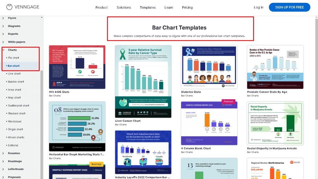
Want to skip the setup? Try one of our customizable bar chart templates to save time and present your data beautifully.
What is a bar chart?
Before I show you how to create a bar graph in Excel, let’s understand some basics first.
A bar graph has two axes — the horizontal X-axis, and the vertical Y-axis. The X-axis showcases categories of data, and the Y-axis is used to present numerical values.
The height of the rectangular bars in a bar graph represents the magnitude of actual data points.
Here’s an example:

However, bar graphs do not convey information about variance or statistical measure that shows the spread of values or the standard deviation.
If you want to include that information, it’s better to consider box plots instead.
For a more comprehensive overview of bar charts, check out this post:
Other factors you’ll want to keep in mind include the labels, which provide a description of what each axis represents and gridlines that can be added to aid interpretation.
I’ve labeled this bar chart with all the information you need to know:

Oh and one more thing.
Though not common, sometimes bar charts can include an additional horizontal or vertical secondary axis when there are more than two sets of data.
For example, let’s say you have a bar graph showing the sales revenue of different products on the primary vertical axis. To show the number of units sold for each product, you might add a secondary vertical axis.
Types of bar charts you can make in Excel
Excel is known for helping people create several types of charts for different presentation needs.
Besides the column chart in Excel, other options include a pie chart, line chart, and scatterplot.
Not sure if a bar chart is the right choice for you? Check out our post on how to choose the best chart for your data to help you decide.
But if you’re confident a bar graph is what you need, the next step is to decide what type of bar chart you want to create.
Excel provides various options for bar charts, including clustered, stacked, floating, and grouped bar charts, as well as histograms.
For example, a stacked bar chart is helpful in comparing percentages or proportions within different categories while a clustered bar chart allows for straightforward comparisons of data across categories.
However, you won’t find each type of bar chart in Excel.
For instance, it’s not possible to create a timeline or schedule bar chart (also known as a Gantt chart) in Excel unless you want to spend hours manually customizing the appearance.
So why not head over to our selection of bar chart templates where you’ll find each of these types of bar charts ready to be made your own in a few clicks?
Now, onto the type bar charts you can create in Excel:
Clustered bar chart
I used to rely on clustered bar charts all the time when comparing department performance across quarters.
Each group of bars sits side by side, so it’s super easy to spot which team outperformed the others in Q2, for example. If you’ve got multiple categories sharing the same metric, this chart’s your go-to.
Excel offers both 2D and 3D clustered bar chart options, which are widely used for data comparison.
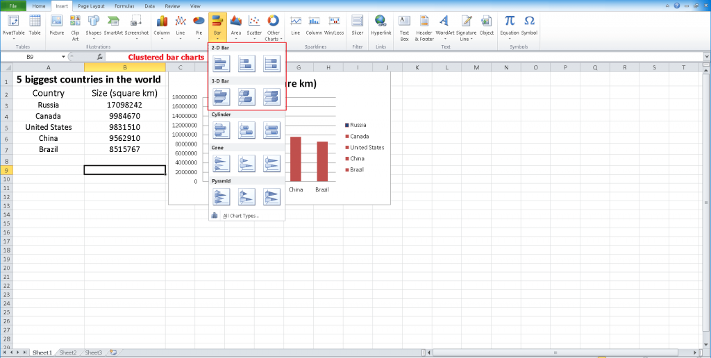
Here’s an example of a clustered bar chart:

Clustered bar charts allow you to add overlapping bars to compare multiple series of data.
In the example above, the adjacent nature of the clustered bars makes it easy to visualize how each cake flavor performs in different cities.
Stacked bar chart – visualizing cumulative totals
In a stacked bar chart, bars are stacked on top of each other to represent the cumulative total of multiple data series.
Each segment within a bar represents a different category or group, and the overall height of the bar represents the total value.
When I was building a report to show overall marketing ROI by channel, the stacked bar chart made things click. It lets you stack segments on top of each other in a single bar, showing both the total and the individual parts. It’s a great way to say, “Here’s the big picture, and here’s how we got there.”
Of course, you can create stacked bar charts in Excel too.
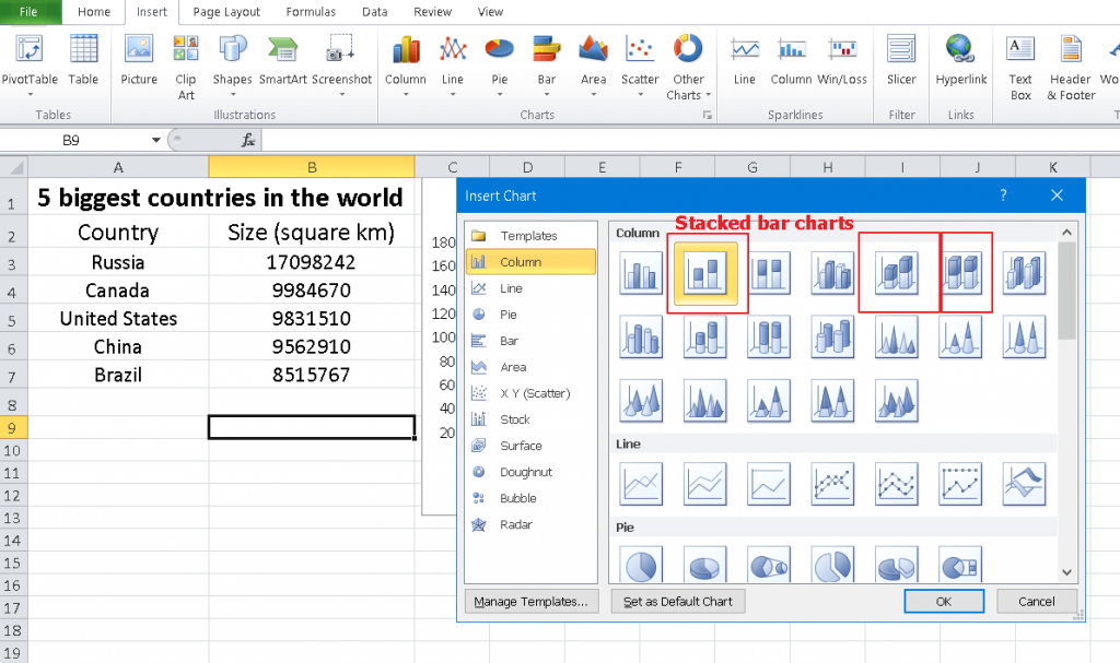
Here’s a real-world example:

Grouped bar chart
Grouped bar charts organize multiple bars within larger category groups, helping you compare subcategories easily.
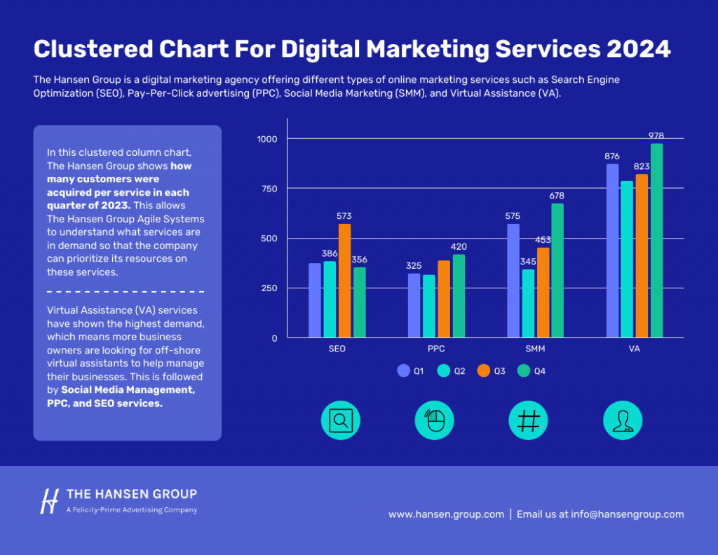
These came in handy when I was tracking how many customers were acquired in each quarter.
Take this clustered column chart template for example, Q1 to Q4 data were grouped under each service, like SEO, PPC and social media management. It was a clear way to show what services are in demand so that the company can prioritize its resources.
Percentage bar chart
A percentage bar chart standardizes all bars to 100%, so you can focus on proportions instead of totals.
I remember presenting a report and watching everyone’s eyes glaze over until I switched to a percentage bar chart.
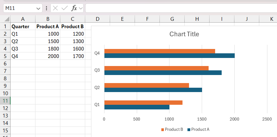
Suddenly, it was clear that Product A had lost ground to B, even though the raw numbers didn’t make it obvious. It’s one of those “why didn’t I do this earlier?” tools.
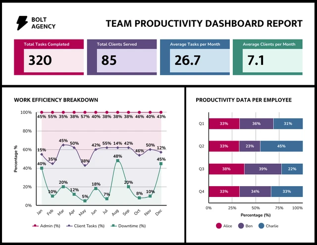
You can visualize this kind of data using this template, which includes clean, customizable charts ideal for highlighting proportional trends, like time allocation or task breakdowns, without overwhelming your audience with raw figures.
Double bar chart
Double bar charts show two bars per category, letting you compare two related data sets side by side.
These are my go-to for before-and-after visuals. Two bars per category, easy to build, even easier to explain. It’s clean, direct and tells a story fast.
Bar chart with 3 variables
Okay, this one takes a bit of creativity. This type of bar chart uses visual tricks like color coding or pivot charts to show a third variable alongside the basic bar data.
I once had to show product sales by region and channel type. One workaround was adding color to represent the third variable using a pivot chart.
Another time, I used varying patterns instead. It’s not perfect, but with the right formatting, it totally works and helps people grasp more complex stories without overwhelming them.
How to make a bar chart in Excel (with screenshots)
Creating a bar chart in Excel is quick and effective for visualizing data. In this tutorial, we’re using Microsoft Excel for Microsoft 365 (Office 365) to ensure compatibility with the latest UI and features.
Follow these four steps to create a clean, professional bar chart from scratch.
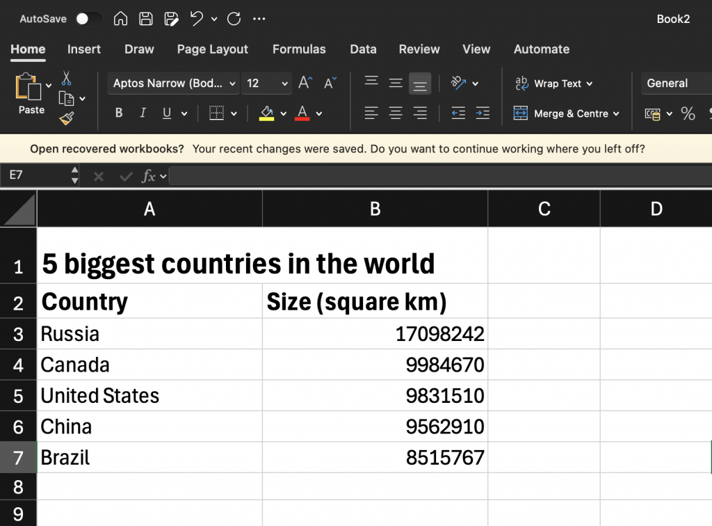
Step 1 – Enter your data in Excel
Start by organizing your data in two columns:
- The first column for categories (e.g. country names)
- The second column for values (e.g. population sizes)
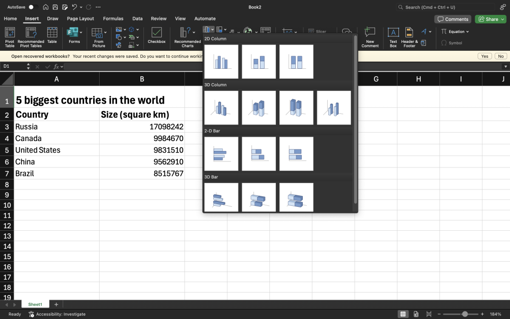
Step 2 – Insert a bar chart from the ribbon
- Select the entire data range, including headers.
- Go to the Insert tab in the ribbon.
- In the Charts group, click the Insert Column or Bar Chart icon.
- Choose a bar chart type—Clustered Bar is a popular option.
Tip: Excel refers to vertical bar charts as “Column Charts” and horizontal ones as “Bar Charts.” Pick the one that suits your layout.
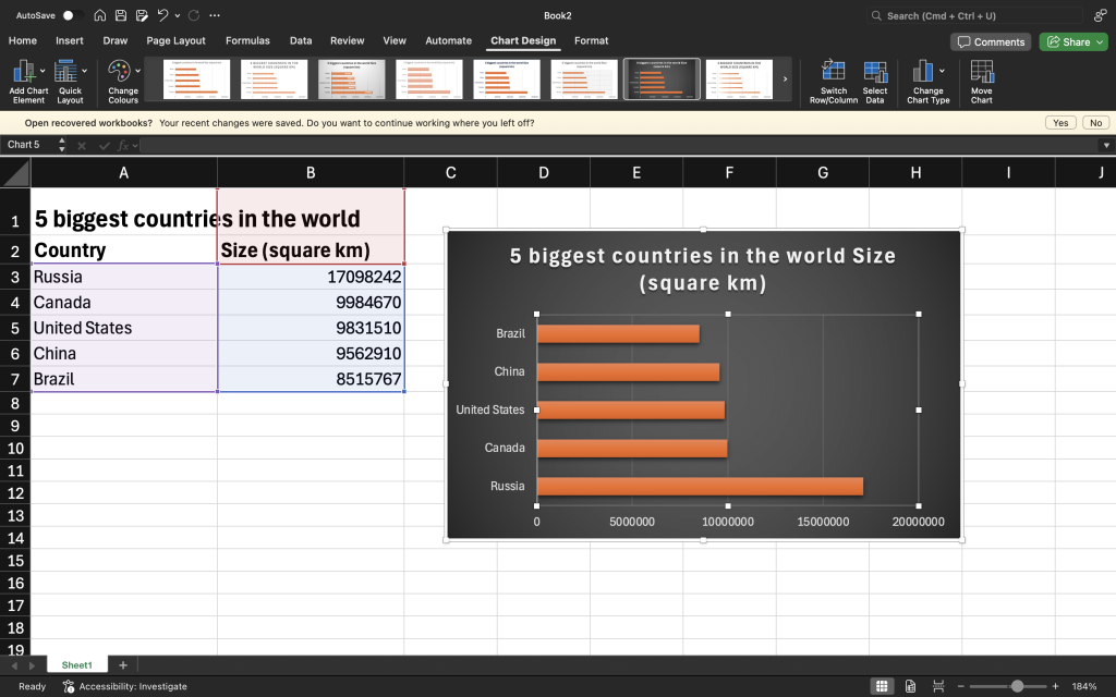
Step 3 – Customize the chart layout and colors
Once the chart appears:
- Click the chart to activate Chart Design and Format tabs.
- Use Chart Styles to apply a pre-designed color theme.
- Click Change Colors to apply your brand palette or a more readable combination.
- Right-click any bar to manually format fill colors, outlines, or add gradients.
For clearer visuals:
- Avoid cluttered color schemes
- Use contrasting colors for high/low values
- Remove unnecessary 3D effects for clean presentation
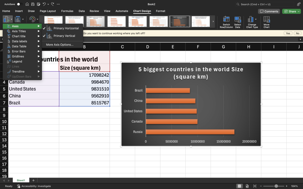
Step 4 – Format labels, axis titles and gridlines
Fine-tune your chart for clarity:
- Click on the chart title to edit it
- Use the Chart Elements (+) button (top right of the chart) to toggle:
- Axis titles
- Data labels
- Gridlines
- Format axis titles for clarity (e.g. “Country” on X-axis, “Population” on Y-axis)
- Adjust data label position (inside or outside bars) for better readability
Tip: Keep your chart minimalist—use only the labels and gridlines that add value. You can also use GPT for Excel to generate and format chart data faster using AI prompts directly inside your spreadsheet.
How to make better bar charts with Venngage
Of course, Excel isn’t the only way to make a column chart.
With limitations in flexibility, customization options, or the ability to edit and collaborate in real time, Excel is not the best way to create bar charts.
With Venngage, you can really elevate your bar charts thanks to our intuitive editor tool and professional bar chart templates that showcase progress and key performance indicators effectively.
Here’s what you need to do:
Step 1 – Sign up for a Venngage account (it’s free!)
Start by signing up for Venngage with your email, Gmail or Facebook account.

Step 2 – Select a template from our library
Venngage has a diverse range of bar chart templates to choose from. Whether you’re looking for stacked bar charts, a vertical bar graph, or a horizontal bar chart, we’ve got templates for you to edit.
For example, here’s a beautiful stacked bar chart you can make your own:

Or this stunning horizontal bar chart.

Step 3 – Edit your bar chart in a few clicks
Have no design experience? No sweat!
All our templates are easy to edit thanks to a drag-and-drop interface.
Swap placeholder data with your own in a spreadsheet interface.
But that’s not all.
Venngage also offers 40,000 icons and illustrations to help you visualize and bring bar charts to life. This will ensure your next assignment, presentation, or report is not dull and grey.
And if you upgrade to a Business account, you can also enjoy My Brand Kit — the one-click branding kit that lets you upload your logo and apply brand colors and fonts to any design.

A business account also includes a real-time collaboration feature, so you can invite members of your team to work simultaneously on a project.
When you upgrade to a Business account, you can download your quote poster as a PNG, PDF, or interactive PDF.
But you can always share your quote poster online for free.
Frequently Asked Questions
How to make a column graph in Excel?
To create a column graph in Microsoft Excel, follow these steps: 1) Enter your data, 2) Select your data range, 3) Insert a column graph, 4) Choose a column chart type, 5) Let Excel create the chart, 6) Customize the bar chart to your needs, and 7) Save and export.
How to make a grouped bar chart in Excel?
To create a grouped bar chart in Excel, follow these steps: 1) Enter your data, 2) Select your data range, 3) Insert a grouped bar chart, 4) Customize your chart, 5) Add axis labels and titles, and 6) Save and export.
How to make a percentage bar graph in Excel?
To create a percentage bar graph in Excel, follow these steps: 1) Enter your data, 2) Calculate your percentages, 3) Select your data range, 4) Insert a clustered column bar chart, 5) Switch to the percentage scale, 6) Customize the chart, 7) Add axis labels and titles, and 8) Save and export.
How to make a bar graph in Excel with 3 variables?
To make a bar graph in Excel with 3 variables, follow these steps: 1) Enter your data, 2) Select your data range, 3) Insert a clustered column chart, 4) Customize your chart, 5) Add axis labels and titles, and 6) Save and export your clustered bar chart.
How to make a double bar graph in Excel?
To create a double bar graph in Excel, follow these steps: 1) Enter your data, 2) Select your data range, 3) Insert a clustered bar chart, 4) Customize your chart, 5) Add axis labels and titles 6) group the bars by right-clicking on a bar and selecting “Format Data Series” from the menu. Here, change “Series Overlap” and “Gap Width” settings to adjust the spacing between the bars to 0 to create a double bar graph, and 7) Save and export.
How do I create a bar chart in Excel with multiple bars?
To create a bar chart in Excel with multiple bars, follow these instructions: 1) Enter your data, 2) Select your data range, 3) Choose the type of bar chart you want to create, 4) Select the “Chart Design” option in the “Data” tab and click on “Switch Row/Column” button, 5) Save and export.
Conclusion
With Venngage, it’s easy to elevate your data visualization game and create stunning bar charts that grab the attention of a reader or audience.
Or you can make boring bar charts with Excel that puts people to sleep.
What choice will you go with?